House price 실습

House Prices - Advanced Regression Techniques | Kaggle

해당 대회 문제를 풀어보자

위의 링크로 들어가면 data_description.txt, sample_submission.csv, test.csv, train.csv 파일들을 받을 수 있다.

각 파일 설명 및 데이터 설명은 다음과 같다.

File descriptions

• train.csv - the training set

• test.csv - the test set

• data_description.txt - full description of each column, originally prepared by Dean De Cock but lightly edited to match the column names used here

• sample_submission.csv - a benchmark submission from a linear regression on year and month of sale, lot square footage, and number of bedrooms

Data fields

Here's a brief version of what you'll find in the data description file.

• SalePrice - the property's sale price in dollars. This is the target variable that you're trying to predict.

• MSSubClass: The building class

• MSZoning: The general zoning classification

• LotFrontage: Linear feet of street connected to property

• LotArea: Lot size in square feet

• Street: Type of road access

• Alley: Type of alley access

• LotShape: General shape of property

• LandContour: Flatness of the property

• Utilities: Type of utilities available

• LotConfig: Lot configuration

• LandSlope: Slope of property

• Neighborhood: Physical locations within Ames city limits

• Condition1: Proximity to main road or railroad

• Condition2: Proximity to main road or railroad (if a second is present)

• BldgType: Type of dwelling

• HouseStyle: Style of dwelling

• OverallQual: Overall material and finish quality

• OverallCond: Overall condition rating

• YearBuilt: Original construction date

• YearRemodAdd: Remodel date

• RoofStyle: Type of roof

• RoofMatl: Roof material

• Exterior1st: Exterior covering on house

• Exterior2nd: Exterior covering on house (if more than one material)

• MasVnrType: Masonry veneer type

• MasVnrArea: Masonry veneer area in square feet

• ExterQual: Exterior material quality

• ExterCond: Present condition of the material on the exterior

• Foundation: Type of foundation

• BsmtQual: Height of the basement

• BsmtCond: General condition of the basement

• BsmtExposure: Walkout or garden level basement walls

• BsmtFinType1: Quality of basement finished area

• BsmtFinSF1: Type 1 finished square feet

• BsmtFinType2: Quality of second finished area (if present)

• BsmtFinSF2: Type 2 finished square feet

• BsmtUnfSF: Unfinished square feet of basement area

• TotalBsmtSF: Total square feet of basement area

• Heating: Type of heating

• HeatingQC: Heating quality and condition

• CentralAir: Central air conditioning

• Electrical: Electrical system

• 1stFlrSF: First Floor square feet

• 2ndFlrSF: Second floor square feet

• LowQualFinSF: Low quality finished square feet (all floors)

• GrLivArea: Above grade (ground) living area square feet

• BsmtFullBath: Basement full bathrooms

• BsmtHalfBath: Basement half bathrooms

• FullBath: Full bathrooms above grade

• HalfBath: Half baths above grade

• Bedroom: Number of bedrooms above basement level

• Kitchen: Number of kitchens

• KitchenQual: Kitchen quality

• TotRmsAbvGrd: Total rooms above grade (does not include bathrooms)

• Functional: Home functionality rating

• Fireplaces: Number of fireplaces

• FireplaceQu: Fireplace quality

• GarageType: Garage location

• GarageYrBlt: Year garage was built

• GarageFinish: Interior finish of the garage

• GarageCars: Size of garage in car capacity

• GarageArea: Size of garage in square feet

• GarageQual: Garage quality

• GarageCond: Garage condition

• PavedDrive: Paved driveway

• WoodDeckSF: Wood deck area in square feet

• OpenPorchSF: Open porch area in square feet

• EnclosedPorch: Enclosed porch area in square feet

• 3SsnPorch: Three season porch area in square feet

• ScreenPorch: Screen porch area in square feet

• PoolArea: Pool area in square feet

• PoolQC: Pool quality

• Fence: Fence quality

• MiscFeature: Miscellaneous feature not covered in other categories

• MiscVal: $Value of miscellaneous feature

• MoSold: Month Sold

• YrSold: Year Sold

• SaleType: Type of sale

• SaleCondition: Condition of sale

이 문제는 타이타닉과 같은 classification 문제가 아닌, Regression 즉 회귀 문제이다. 정답을 실수 형태로 예측하는 문제이다.

풀이 방법은 House price Predictions 블로그를 따라풀어보았다.

1. 데이터 로드

import pandas as pd
import numpy as np
from scipy.stats import norm
%matplotlib inline
import matplotlib.pyplot as plt
import seaborn as sns
import warnings; warnings.simplefilter('ignore')

train=pd.read_csv('../input/house-prices-advanced-regression-techniques/train.csv',index_col='Id')
test=pd.read_csv('../input/house-prices-advanced-regression-techniques/test.csv',index_col='Id')
submission=pd.read_csv('../input/house-prices-advanced-regression-techniques/sample_submission.csv',index_col='Id')
data=train
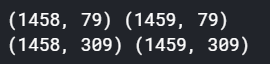
print(train.shape, test.shape, submission.shape)

패키지들을 로드하고, 데이터를 불러온다.

결과를 보면 1460행의 train data, 1459행의 test data의 집값을 예측해야함을 확인 할 수 있다. 이때 변수는 80개, 79개이다.

2. 데이터 분석

1) 타겟 변수 확인 (Distribution of Target)

figure, (ax1, ax2) = plt.subplots(nrows=1, ncols=2)
figure.set_size_inches(14,6)
sns.distplot(data['SalePrice'], fit=norm, ax=ax1)
sns.distplot(np.log(data['SalePrice']+1), fit=norm, ax=ax2)

집값을 타겟 변수로 잡는다.

다음과 같은 그래프를 확인 할 수 있는데, 왼쪽의 그래프를 보면 많은 데이터들이 중심 값인 400000 보다 왼쪽으로 치우친 'Left Skewness' 상태, 즉 왜도 상태임을 확인 할 수 있다. 비대칭이 심하면 머신러닝 알고리즘이 학습을 잘 하지 못하는 방해요소가 되므로, 변수에 로그를 취해 정규분포에 가깝게 만든다.

로그에 +1을 해주는 이유는 log0의 값은 마이너스 무한대로 발산하기 때문에 이를 방지하기 위해서이다. (log lp)

오른쪽의 그래프는 로그를 취한 값으로, 머신러닝에게 로그를 취한 값을 타겟 변수로 주어 예측하게 한 후 제출 할 때만 지수 계산을 해서 제출한다.

2) 변수간 상관관계 확인

corr=data.corr()
top_corr=data[corr.nlargest(40,'SalePrice')['SalePrice'].index].corr()
figure, ax1 = plt.subplots(nrows=1, ncols=1)
figure.set_size_inches(20,15)
sns.heatmap(top_corr,annot=True,ax=ax1)

위의 그래프는 타겟 변수인 'SalePrice'와 가장 큰 상관관계를 가진 40개의 변수를 표시하는 그래프이다.

변수 'OverallQual'이라는 변수가 상관계수 0.79로 타겟변수와 가장 큰 상관관계를 가지고 있음을 확인 할 수 있다. 전반적으로 OverallQual이 증가하면 집값도 증가한다고 볼 수 있다. 두번째로는 GriLivArea 가 0.71로 상관계수를 가짐을 볼 수 있다.

sns.regplot(data['GrLivArea'], data['SalePrice'])

GriLivArea와 SalePrice의 관계를 표시한 그래프는 다음과 같다. 전반적으로 GriLivArea가 증가하면 집값도 증가함을 확인 할 수 있다. 그래프 상 아래쪽 점 두개를 제외하면 점들의 분포는 그래프상의 직선으로 표시가 가능하므로, 두개의 데이터들을 '이상치' (Outlier)로 간주하게 삭제해 머신러닝의 정확도를 높인다.

train=train.drop(train[(train['GrLivArea']>4000) & (train['SalePrice']<300000)].index)

이제 train 와 test를 묶어 add_data라는 변수에 저장후 처리한 후, 학습시키기 전에 잘라 사용한다.

Ytrain=train['SalePrice']
train=train[list(test)]
all_data=pd.concat((train,test), axis=0)
print(all_data.shape)
Ytrain=np.log(Ytrain+1)

타겟 변수를 Ytrain으로 저장하고 로그를 씌운다.

3) 전체 데이터에서 결측지 확인

집에 해당 시설물이 없는 경우는 결측치로 처리되어 있기 때문에 결측치를 처리한다.

cols=list(all_data)
for col in list(all_data):
    if(all_data[col].isnull().sum()) == 0:
        cols.remove(col)
    else:
        pass
print(len(cols))

list(all_data)를 사용해 all_data 열 이름을 리스트로 만든다. 반복문을 통해 all_data에서 해당 열에 결측지가 없으면 리스트에서 그 열을 지워 결측치가 있는 변수의 이름만 남긴다.현재 34개의 행에 결측치가 존재함을 알 수 있다.

리스트에 남아있는 행들의 이름은 위와 같이 print로 출력해 확인 할 수 있다.이 항목들의 결측치를 채우는데, 범주형 변수는 집에 해당 시설물이 없는 경우 'None'이라는 문자열로 채운다.수치형 변수의 경우에는 결측치를 0으로 채운고, 해당 시설물이 없다고 보기 힘든 경우 (외벽 시설, 거래타입 등)에는 결측치를 해당 열의 최빈값으로 채운다.

for col in('PoolQC', 'MiscFeature', 'Alley', 'Fence', 'FireplaceQu', 'GarageType', 'GarageFinish', 'GarageQual', 'GarageCond', 'BsmtQual' ,'BsmtCond', 'BsmtExposure', 'BsmtFinType1', 'BsmtFinType2', 'MasVnrType', 'MSSubClass'):
    all_data[col] = all_data[col].fillna('None')

for col in('GarageYrBlt', 'GarageArea', 'GarageCars', 'BsmtFinSF1', 'BsmtFinSF2', 'BsmtUnfSF', 'TotalBsmtSF', 'BsmtFullBath', 'BsmtHalfBath', 'MasVnrArea', 'LotFrontage'):
    all_data[col] = all_data[col].fillna(0)
    
for col in ('MSZoning', 'Electrical', 'KitchenQual', 'Exterior1st', 'Exterior2nd', 'SaleType', 'Functional', 'Utilities'):
    all_data[col] = all_data[col].fillna(all_data[col].mode()[0])
    
print(f"Total count of missing values in all_data : {all_data.isnull().sum().sum()}")

결측치를 모두 채운 후 missing value를 출력하면 0이 나옴을 확인 할 수 있다.

4) 본격적 데이터 분석 (EDA)

새로운 변수를 만든다. (1) 총 가용 면적

figure, ((ax1,ax2), (ax3,ax4)) = plt.subplots(nrows=2, ncols=2)
figure.set_size_inches(14,10)
sns.regplot(data['TotalBsmtSF'], data['SalePrice'], ax=ax1)
sns.regplot(data['1stFlrSF'], data['SalePrice'], ax=ax2)
sns.regplot(data['2ndFlrSF'], data['SalePrice'], ax=ax3)
sns.regplot(data['TotalBsmtSF']+data['1stFlrSF']+data['2ndFlrSF'], data['SalePrice'], ax=ax4)

지하실, 1층, 2층 면접을 합한 '총 면적' 의 변수를 추가로 만든다. 오른쪽 아래의 그래프가 나머지 3개를 합한 그래프이다.이 그래프를 통해 총 면적이 증가하면 집값이 더 비싸진다고 볼 수 있으며, 상관관계가 꽤 높음을 확인 할 수 있다.

all_data['TotalSF']=all_data['TotalBsmtSF']+all_data['1stFlrSF']+all_data['2ndFlrSF']
all_data['No2ndFlr'] = (all_data['2ndFlrSF']==0)
all_data['NoBsmt'] = (all_data['TotalBsmtSF']==0)

총 면적을 더해 TotalSF 라는 변수로 저장한다. 또한 2층이 없음, 지하실 없음 여부를 나타낼 수 있도록 변수를 추가한다.x값이 0 인 값들 때문에 그래프가 지저분하게 나타나므로 나중에 빼기 위해 따로 저장한다.

(2) 총 욕실 수

figure, ((ax1,ax2), (ax3,ax4)) = plt.subplots(nrows=2, ncols=2)
figure.set_size_inches(14,10)
sns.barplot(data['BsmtFullBath'], data['SalePrice'], ax=ax1)
sns.barplot(data['FullBath'], data['SalePrice'], ax=ax2)
sns.barplot(data['BsmtHalfBath'], data['SalePrice'], ax=ax3)
sns.barplot(data['HalfBath'], data['SalePrice'], ax=ax4)

figure, (ax5) = plt.subplots(nrows=1, ncols=1)
figure.set_size_inches(14,6)
sns.barplot(data['BsmtFullBath']+data['FullBath']+ (data['BsmtHalfBath']/2) + (data['HalfBath']/2), data['SalePrice'], ax=ax5)

욕실 갯수는 총 4개의 열로 이루어져있는데, 이들을 모두 더해 하나로 만든다. FullBath는 욕조 및 샤워시설이 포함되어 있으므로 1개로 카운트, HalfBath는 간단한 욕실이므로 0.5로 카운트해서 더한다.

욕실 수가 더 많을수록 값이 비싸짐을 확인 할 수 있다.욕실이 5개, 6개인 집은 편차 (검정 세로 선)이 없음을 볼 수 있는데, 이는 이 값이 하나씩만 존재한다는 것을 의미한다. 그러므로 이들을 outlier로 판단하고 지운다.

all_data['TotalBath'] = all_data['BsmtFullBath']+all_data['FullBath']+ (all_data['BsmtHalfBath']/2)+ (all_data['HalfBath']/2)

(3) 건축연도 + 리모델링 연도

figure,(ax1,ax2,ax3) = plt.subplots(nrows=1, ncols=3)
figure.set_size_inches(18,8)
sns.regplot(data['YearBuilt'], data['SalePrice'], ax=ax1)
sns.regplot(data['YearRemodAdd'], data['SalePrice'], ax=ax2)
sns.regplot((data['YearBuilt']+data['YearRemodAdd'])/2, data['SalePrice'], ax=ax3)

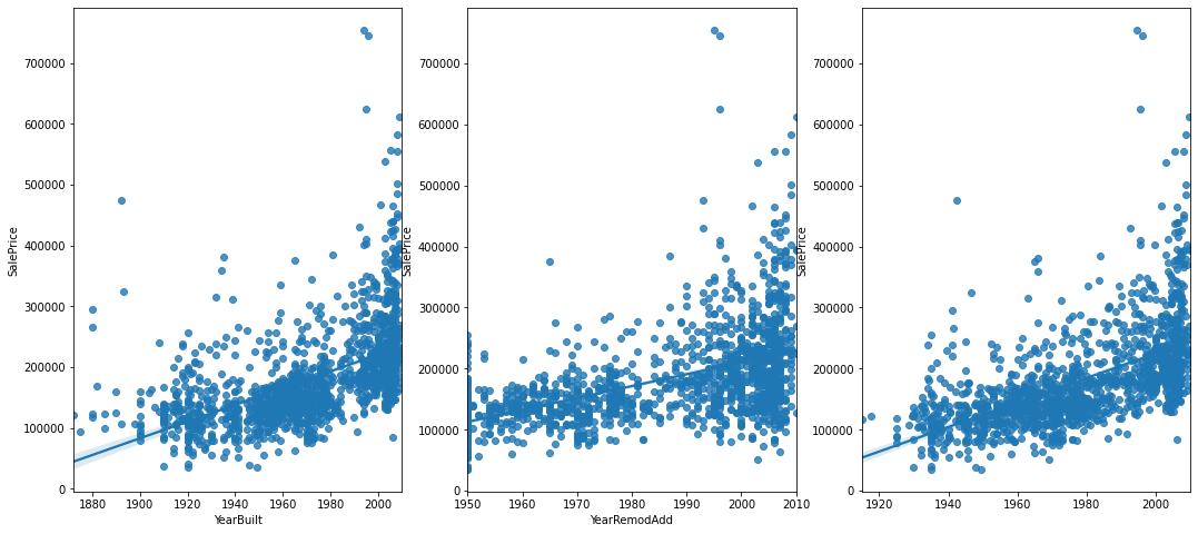
두개의 데이터를 모두 포함하는 데이터를 추가한다. 값이 높은 집들은 지어지지 얼마 되지 않은 신축건물 + 최근에 리모델링까지 함 에 가깝기 때문에 그래프를 합친다.가장 오른쪽 그래프가 두 그래프를 합쳐 평균낸 그래프이다.

all_data['YrBltAndRemod']= all_data['YearBuilt']+all_data['YearRemodAdd']

이를 합친 변수로 저장한다.

5) 자료형 수정

all_data['MSSubClass']= all_data['MSSubClass'].astype(str)
all_data['MoSold'] = all_data['MoSold'].astype(str)
all_data['YrSold'] = all_data['YrSold'].astype(str)

MsSubClass 의 자료들은 숫자로 되어있지만 범주형 변수이기 때문에 문자열로 바꾸어준다.

6) 지하실 점수

집의 시설물들을 묶어서 점수를 매겨보자.

Basement = ['BsmtCond', 'BsmtExposure', 'BsmtFinSF1', 'BsmtFinSF2', 'BsmtFinType1', 'BsmtFinType2', 'BsmtQual', 'BsmtUnfSF', 'TotalBsmtSF']
Bsmt = all_data[Basement]

먼저 지하실에 관한 변수들을 묶어서 저장한다.

Bsmt=Bsmt.replace(to_replace='Po', value=1)
Bsmt=Bsmt.replace(to_replace='Fa', value=2)
Bsmt=Bsmt.replace(to_replace='TA', value=3)
Bsmt=Bsmt.replace(to_replace='Gd', value=4)
Bsmt=Bsmt.replace(to_replace='Ex', value=5)
Bsmt=Bsmt.replace(to_replace='None', value=0)

Bsmt=Bsmt.replace(to_replace='No', value=1)
Bsmt=Bsmt.replace(to_replace='Mn', value=2)
Bsmt=Bsmt.replace(to_replace='Av', value=3)
Bsmt=Bsmt.replace(to_replace='Gd', value=4)

Bsmt=Bsmt.replace(to_replace='Unf', value=1)
Bsmt=Bsmt.replace(to_replace='LwQ', value=2)
Bsmt=Bsmt.replace(to_replace='Rec', value=3)
Bsmt=Bsmt.replace(to_replace='BLQ', value=4)
Bsmt=Bsmt.replace(to_replace='ALQ', value=5)
Bsmt=Bsmt.replace(to_replace='GLQ', value=6)

이들을 인코딩한다. 위의 값들은 data description 텍스트파일에 있으며, 좋은 값일수록 높은숫자를 부여한다.지하실이 없으면 0을 입력한다.

Bsmt['BsmtScore'] = Bsmt['BsmtQual']*Bsmt['BsmtCond']*Bsmt['TotalBsmtSF']
all_data['BsmtScore'] = Bsmt['BsmtScore']

Bsmt['BsmtFin'] = (Bsmt['BsmtFinSF1']*Bsmt['BsmtFinType1']) + (Bsmt['BsmtFinSF2']*Bsmt['BsmtFinType2'])
all_data['BsmtFinScore'] = Bsmt['BsmtFin']
all_data['BsmtDNF'] = (all_data['BsmtFinScore']==0)

몇개 항목들을 곱해 지하실의 전반적인 상태를 복합적으로 평가할 수 있는 변수를 만든다.'BsmtFinScore' 은 지하실의 완성도 점수, 'BsmtScore'은 지하실의 종합 점수, 'BsmtDNF'는 지하실의 미완성 여부를 나타내는 변수이다.

7) 토지 점수

lot=['LotFrontage', 'LotArea', 'LotConfig', 'LotShape']
Lot=all_data[lot]

Lot['LotScore'] = np.log((Lot['LotFrontage']*Lot['LotArea'])+1)

all_data['LotScore']=Lot['LotScore']

비슷한 상태의 토지면적과 모양, 접근성 등을 고려할 수 있는 점수를 만들어 변수로 저장한다.

8) 차고 점수

garage=['GarageArea', 'GarageCars', 'GarageCond', 'GarageFinish', 'GarageQual', 'GarageType', 'GarageYrBlt']
Garage = all_data[garage]
all_data['NoGarage'] = (all_data['GarageArea']==0)

Garage=Garage.replace(to_replace='Po', value=1)
Garage=Garage.replace(to_replace='Fa', value=2)
Garage=Garage.replace(to_replace='TA', value=3)
Garage=Garage.replace(to_replace='Gd', value=4)
Garage=Garage.replace(to_replace='Ex', value=5)
Garage=Garage.replace(to_replace='None', value=0)

Garage=Garage.replace(to_replace='Unf', value=1)
Garage=Garage.replace(to_replace='RFn', value=2)
Garage=Garage.replace(to_replace='Fin', value=3)

Garage=Garage.replace(to_replace='CarPort', value=1)
Garage=Garage.replace(to_replace='Basment', value=4)
Garage=Garage.replace(to_replace='Detchd', value=2)
Garage=Garage.replace(to_replace='2Types', value=3)
Garage=Garage.replace(to_replace='Basement', value=5)
Garage=Garage.replace(to_replace='Attchd', value=6)
Garage=Garage.replace(to_replace='BuiltIn', value=7)

Garage['GarageScore']=(Garage['GarageArea'])*(Garage['GarageCars'])*(Garage['GarageFinish'])*(Garage['GarageQual'])*(Garage['GarageType'])
all_data['GarageScore']=Garage['GarageScore']

같은 방법으로 차고의 종합 점수를 판단할 수 있도록 실행한다.

9) 기타 변수

all_data=all_data.drop(columns=['Street', 'Utilities', 'Condition2', 'RoofMatl', 'Heating'])

비정상적으로 하나의 값만 많은 변수들을 삭제한다.또한 비정상적으로 빈 값이 많은 변수들을 삭제한다.

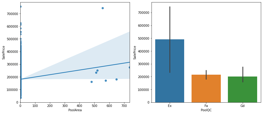
figure, (ax1,ax2) = plt.subplots(nrows=1, ncols=2)
figure.set_size_inches(14,6)
sns.regplot(data=data, x='PoolArea', y='SalePrice', ax=ax1)
sns.barplot(data=data, x='PoolQC', y= 'SalePrice', ax=ax2)

수영장이 있는 집 그래프

all_data=all_data.drop(columns=['PoolArea', 'PoolQC'])

figure, (ax1,ax2) = plt.subplots(nrows=1, ncols=2)
figure.set_size_inches(14,6)
sns.regplot(data=data, x='MiscVal', y='SalePrice', ax=ax1)
sns.barplot(data=data, x='MiscFeature', y='SalePrice', ax=ax2)

테니스코트 있는 집 그래프

all_data=all_data.drop(columns=['MiscVal', 'MiscFeature'])

해당 값들을 삭제한다.

채워진 결측치가 많은 경우

sns.regplot(data=data, x='LowQualFinSF', y='SalePrice')
sns.regplot(data=data, x='OpenPorchSF', y='SalePrice')
sns.regplot(data=data, x='WoodDeckSF', y='SalePrice')

(위부터 순서대로)

0값만 분리한다.

all_data['NoLowQual']=(all_data['LowQualFinSF']==0)
all_data['NoOpenPorch']=(all_data['OpenPorchSF']==0)
all_data['NoWoodDeck']=(all_data['WoodDeckSF']==0)

3. 전처리

1) 범주형 변수

non_numeric=all_data.select_dtypes(np.object)

def onehot(col_list):
    global all_data
    while len(col_list) != 0:
        col=col_list.pop(0)
        data_encoded=pd.get_dummies(all_data[col], prefix=col)
        all_data=pd.merge(all_data, data_encoded, on='Id')
        all_data=all_data.drop(columns=col)
    print(all_data.shape)
    
onehot(list(non_numeric))

범주형 데이터를 숫자로 인코딩하면 제대로 되지 않을 수 있기 때문에 일단 원핫 인코딩을 한다.

2) 수치형 변수

비대칭이 너무 심해지지 않게 Right Skewed가 크게 되어있는 데이터들에만 로그를 씌운다.

numeric=all_data.select_dtypes(np.number)

def log_transform(col_list):
    transformed_col=[]
    while len(col_list)!=0:
        col=col_list.pop(0)
        if all_data[col].skew() > 0.5:
            all_data[col] = np.log(all_data[col]+1)
            transformed_col.append(col)
        else:
            pass
    print(f"{len(transformed_col)} features had been transformed")
    print(all_data.shape)
    
log_transform(list(numeric))

이제 데이터들을 나눈다. all_data항목을 test 데이터의 개수에 맞게끔 잘라서 따로 저장한다.

print(train.shape, test.shape)
Xtrain=all_data[:len(train)]
Xtest=all_data[len(train):]
print(Xtrain.shape, Xtest.shape)

원래 train 데이터의 개수와 데이터를 가공한 Xtrain 데이터의 개수가 1458개로 동일함을 확인 할 수 있다.

4. 머신러닝 모델로 학습

from sklearn.linear_model import ElasticNet, Lasso
from sklearn.ensemble import GradientBoostingRegressor
from sklearn.pipeline import make_pipeline
from sklearn.preprocessing import RobustScaler
from xgboost import XGBRegressor
import time
import optuna
from sklearn.model_selection import cross_val_score
from sklearn.metrics import mean_squared_error

model_Lasso=make_pipeline(RobustScaler(), Lasso(alpha=0.000327, random_state=18))
model_ENet = make_pipeline(RobustScaler(), ElasticNet(alpha=0.00052, l1_ratio=0.70654, random_state=18))
model_GBoost = GradientBoostingRegressor(n_estimators=3000, learning_rate=0.05, max_depth=4, max_features='sqrt', min_samples_leaf=15, min_samples_split=10, loss='huber', random_state=18)
model_XGB=XGBRegressor(colsample_bylevel=0.9229733609038979, colsample_bynode=0.21481791874780318, colsample_bytree=0.067964318297635, gamma=0.8989889254961725, learning_rate=0.009192310189734834, max_depth=3, n_estimators=3602, reg_alpha=3.185674564163364e-12, reg_lambda=4.95553539265423e-13, seed=18, subsample=0.8381904293270576, tree_method='gpu_hist', verbosity=0)

4개의 모델을 불러와서 저장한다. 최종 예측 결과물은 4개 모델의 예측값을 평균값을 사용한다.

model_Lasso.fit(Xtrain, Ytrain)
Lasso_predictions=model_Lasso.predict(Xtest)
train_Lasso=model_Lasso.predict(Xtrain)

model_ENet.fit(Xtrain, Ytrain)
ENet_predictions=model_ENet.predict(Xtest)
train_ENet=model_ENet.predict(Xtrain)

model_XGB.fit(Xtrain, Ytrain)
XGB_predictions=model_XGB.predict(Xtest)
train_XGB=model_XGB.predict(Xtrain)

model_GBoost.fit(Xtrain, Ytrain)
GBoost_predictions=model_GBoost.predict(Xtest)
train_GBoost=model_GBoost.predict(Xtrain)

log_train_predictions= (train_Lasso + train_ENet + train_XGB + train_GBoost)/4
train_score = np.sqrt(mean_squared_error(Ytrain, log_train_predictions))
print(f"Scoring with train data: {train_score}")

log_predictions= (Lasso_predictions+ ENet_predictions + XGB_predictions + GBoost_predictions)/4
predictions = np.exp(log_predictions)-1
submission['SalePrice'] = predictions
submission.to_csv('Result.csv')